The Leak Frequencies Decide Your QRA Before Any Modelling

Most arguments about a quantitative risk assessment are arguments about dispersion. Which model, which stability class, whether the cloud was allowed to slump properly. Those are worth having. They are also downstream of the number that already fixed the answer.

Release frequency enters the result linearly. Halve it and you halve the risk. There is no damping, no square root, no averaging that softens it. A study that took its frequencies from a table without asking whether the table describes your plant has made its most consequential decision before anyone opened the software.

f_{re l e a se} = j \sum n_{j} λ_{j} I R = i \sum f_{re l e a se, i}; P_{i g n, i}; P_{f, i}

$n_{j}$: count of equipment items of type j inside the isolatable section
$λ_{j}$: generic release frequency per item per year for that type
$P_{i g n}$: probability the release finds an ignition source
$P_{f}$: probability of fatality given the outcome

Every term multiplies. A factor of three in the frequency is a factor of three in the risk, and it survives all the way to the contour on the drawing.

Where the numbers actually come from

Almost nobody derives release frequencies from their own plant history, and for good reason. A single site does not suffer enough leaks to build a statistically meaningful rate. So the industry uses pooled generic data, and there are a handful of sources that most studies draw on.

IOGP Report 434 in its risk assessment data directory series, which pools process release data across a large operator population and is the common reference for oil and gas.
The UK Health and Safety Executive hydrocarbon releases database, built from mandatory offshore reporting, which is unusually well populated because reporting was compulsory rather than voluntary.
The Purple Book, CPR 18E, which carries generic failure frequencies used widely for onshore installations in the Netherlands and by extension across European land use planning work.
Vendor and operator in house datasets, which are sometimes better matched to the equipment but rarely open to scrutiny.

These are not interchangeable. They were assembled from different equipment populations, in different services, under different reporting thresholds, and they are counting slightly different things. Two competent engineers can produce risk results that differ by a large multiple purely by opening different reference documents, and both can defend the choice.

Caution

A reporting threshold is not a physical threshold. A database built on mandatory reporting above a certain release mass will show a lower frequency of small leaks than one built on maintenance records, not because small leaks are rarer but because nobody had to write them down. Comparing across sources without checking what each counted is how order of magnitude errors get in.

Hole size binning, where a lot of the answer hides

Releases do not come in four sizes. Studies model them that way because you cannot run a continuum, so the total frequency for an item gets apportioned across representative hole sizes, typically something like a few millimetres, a few tens of millimetres, and full bore rupture.

That apportionment matters more than it looks. Small holes are far more frequent but produce short hazard ranges. Ruptures are rare but reach the fence. Move a little frequency from the small bin into the large bin and the individual risk contour moves outward, even though the total release frequency has not changed at all.

f_{t o t a l} = k \sum f_{k} with Q_{k} \propto C_{d} A_{k} 2 ρ Δ P

$f_{k}$: frequency assigned to hole size bin k
$A_{k}$: hole area for that bin, which scales with the square of diameter
$C_{d}$: discharge coefficient
$Q_{k}$: release rate driving the hazard range for that bin

Release rate scales with hole area, so with diameter squared. The bin boundaries are therefore a modelling choice with a large lever on the result.

Ask which bin structure was used and where the boundaries sit. If a study used four bins and a reviewer used three, their results are not comparable and neither is wrong.

The parts count, and the error that recurs

Generic frequencies are per item or per metre, so somebody has to count the items. This is mechanical work, usually done late, often by whoever is available, and it is where the most common serious error in a QRA lives.

Counting from a process flow diagram rather than the piping and instrumentation diagrams, which misses most of the small bore connections, drains, vents and instrument tappings that dominate small leak frequency.
Getting the isolatable section boundaries wrong, so the inventory that can actually be released is over or under stated. The section is defined by what closes on demand, not by what appears on one drawing sheet.
Forgetting that small bore connections carry a frequency per connection that is not negligible when there are hundreds of them.
Counting the design intent rather than the plant as built, on a facility that has had twenty years of modifications.

Assumption

Every generic frequency carries an implied population. It assumes equipment of a certain vintage, inspected at a certain frequency, in a certain service severity. Applying it unchanged to a twenty five year old line in wet sour service with a deferred inspection history is an assumption, not a neutral default. State it as one.

A worked comparison

The following is illustrative rather than a project record, and the numbers are round to keep the arithmetic visible. Take one isolatable section containing 120 metres of process pipework, 40 flanged joints, 8 valves and 2 pump seals.

Assess it with dataset A and the summed release frequency comes to 2 in 100 per year. Assess the same section with dataset B, which counted small releases differently and assigns a higher rate to flanged joints, and it comes to 6 in 100 per year. Nothing physical changed. No valve was added. The consequence modelling that follows is identical in both cases.

The individual risk at the nearest occupied building is three times higher in the second study. If your tolerability criterion sits between the two, one study says build and the other says redesign, and the entire difference is a reference document choice made in the first week.

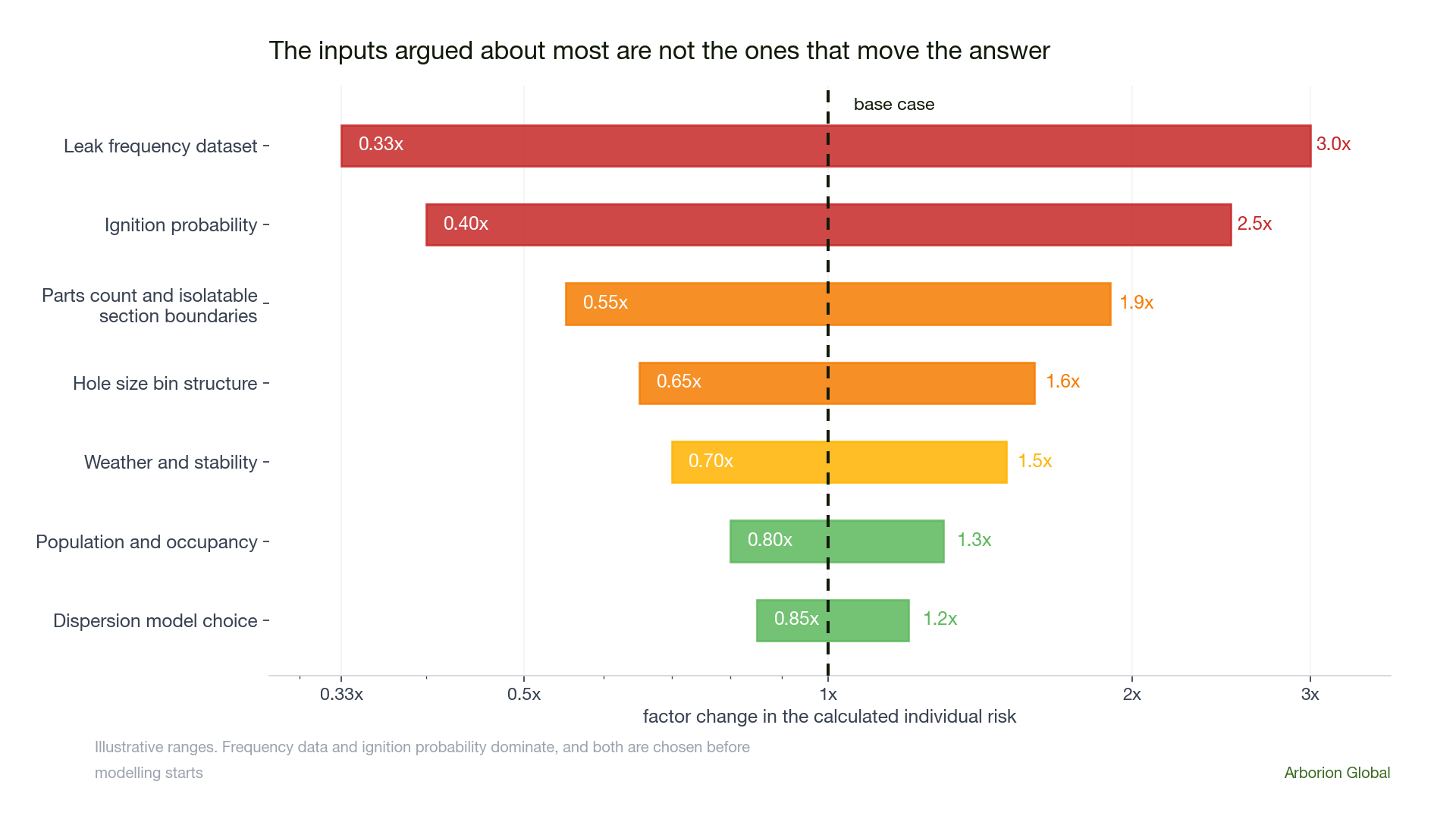
Horizontal bar chart showing the factor by which a quantitative risk assessment result changes across the plausible range of each input, with leak frequency and ignition probability producing the largest swings and dispersion model choice the smallest — Plausible ranges for each input, and what each does to the final risk number. The inputs that get argued about most are not the ones that move the answer most.

This is the reason a sensitivity study is not an optional appendix. If the result is not tested against the range of defensible frequency data, the study has reported one point from a wide distribution and called it the risk.

Adjusting generic data honestly

The answer is not to abandon generic data. It is to say what you did to it and why. Three adjustments are defensible when they are documented and evidenced.

Service severity. Corrosive, erosive, cyclic or sour service justifies an upward adjustment, and the evidence is your own inspection findings rather than a feeling.
Inspection and maintenance quality. A credible risk based inspection programme with closed out findings supports the generic rate. A backlog of deferred inspections does not.
Design and vintage. Welded construction rather than flanged, and modern rather than legacy specification, changes the population you belong to.

What is not defensible is an unstated adjustment, or selecting the dataset that produces the answer the project needs. Both happen, and both are visible to anyone who checks the workings.

What to demand in the study

The frequency source named, with the edition, and the reason it was chosen for this asset.
The parts count, traceable to the piping and instrumentation diagrams, with the isolatable section boundaries drawn.
The hole size bin structure and boundaries stated explicitly.
Any adjustment to generic rates, with the evidence behind it.
A sensitivity case run on the frequency data, not only on the weather.

Reference

IOGP risk assessment data directory, report 434 series, for process release frequencies. UK HSE hydrocarbon releases database for offshore release statistics. Purple Book CPR 18E for generic failure frequencies used in land use planning. CCPS Guidelines for Chemical Process Quantitative Risk Analysis for the overall method. Editions change and so do the numbers, so cite the edition you used.

Three questions worth asking today

Which frequency dataset does our last QRA use, and does anyone on the team know why that one?
Was the parts count done from the piping and instrumentation diagrams or from a flow diagram?
If we reran the study with the other common dataset, would our decision change?

If the answer to the third is yes, you do not have a risk result. You have one sample from a distribution, and the decision it supports needs to be made on the range rather than the point.

Related services

All insights Talk to a specialist